Classifiers

Introduction

Classifiers are the essence of our tool. They define how the signal processing pipeline looks and can be used to translate raw biosensor data into meaningful values.

By default, no classifier is loaded when Studio starts. The exception is the product tour, which opens an example classifier and state machine when it runs.

To load a classifier from the neuromore cloud, double-click it in the Back-End File System window. A single click only selects it. If you can edit the file, you can also right-click it and choose Open. You can’t load a file while a session is running.

File system

This section shows how to create folders and classifiers, and how to edit and save them.

Folders and permissions

Your personal folder holds your own files. Other folders can be shared, and they show a different icon. A shared folder lets people with access work with the same files.

Each file and folder has its own permissions for create, read, update, execute and delete. These decide which buttons are active and which context menu entries you see. Opening a file needs the execute permission. Without it, nothing opens and no message appears.

To edit a read-only classifier, right-click it and choose Copy To Personal Folder. Then edit your copy.

Create a classifier

1. In the Back-End File System window, select a folder you can write to, such as your personal folder.
2. To put the classifier in a new folder, click the Create new folder button and enter a name. Then select the new folder.
3. Click the Create new file button, or right-click the folder and choose Create File.
4. Enter a name, choose Classifier in the type list and click Ok.
5. Double-click the new file. It opens in the Classifier window.
6. Add nodes and connections, as described in Edit a graph.
7. Click the Save button on the toolbar of the Classifier window.

Save your work before you exit. The context menu in the file system has no save entry for this, and the dialog shown when you exit with unsaved changes offers only Discard or Cancel.

Edit a graph

• Open the palette and attributes: click the Tools button at the top right of the Classifier window. The panel shows the node palette and the attributes of the selected node.
• Add a node: drag it from the palette onto the graph, or right-click the graph and choose Add Node.
• Connect two nodes: drag from an output port to an input port.
• Remove a node or connection: select it, then press Delete (Backspace on macOS), or right-click and choose Remove Node or Remove Connection.

Context menu

Right-click an item in the Back-End File System window to see what you can do with it. The entries depend on the item type and your permissions. These are the main ones:

• Files: Open, Rename File, Copy To Personal Folder, Delete File, Copy JSON to clipboard, Download, Upload, Revisions.
• Folders: Create Folder, Create File, Rename Folder, Delete Folder.

In 1.7.3: The file entries Download and Upload are called Save To HDD and Upload local file to cloud.

The neuromore cloud has a built-in revision system. To open an earlier version of a classifier, right-click the file, choose Revisions and pick a revision number.

Vocabulary

Some definitions that might come in handy for the remainder of this document.

Classifier

We call classifiers the complete system from data acquisition to outputs. The name classifier comes from the machine learning lingo, where classifiers are algorithms that take in data and assign that data a most probable label or class. While neuromore can be used to create many systems that are not classifiers, conceptually, they are one of the most useful systems that neuromore aims to create.

Graphs

neuromore uses visual programming to facilitate the creation of classifiers. In particular, neuromore uses connected graphs that allow users to ‘code’ data processing routines more intuitively.

Nodes

Graphs are made up of interconnected nodes. These nodes act like engineering ‘black boxes’ that allow users to create functioning graphs just by knowing what individual nodes do, without needing to understand how they do it. The Nodes page describes the inputs, outputs and function of each node.

Basic Classifier Structure

This example is a minimal classifier that shows the main structural components of a graph:

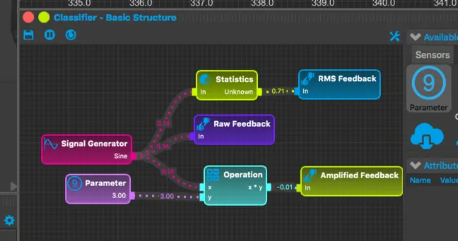
Input: Two nodes from the Input category feed the graph.

• A Signal Generator produces a sine wave with its default settings (Frequency = 1 Hz, Amplitude = 1).
• A Parameter holds the amplification factor. Set its Value to 3.

Processing: The processing logic computes an amplified (3x) version of the input and the RMS value of the signal. Both nodes are in the Math category, and neither does this with its default settings.

• Operation: Set Math Function to Multiply (the default is Add). Connect the Signal Generator to x and the Parameter to y. Both inputs must have the same sample rate. The Signal Generator runs at 128 Hz by default, and a Parameter with its default Sample Rate of 0 takes the rate of the active device. With a real device at another rate, Operation shows “Input sample rates are incompatible.” To avoid this, disconnect real devices or set the Parameter’s Sample Rate to 128.
• Statistics: Set Statistic to RMS (the default is Mean). Connect the Signal Generator to In. The output port of this node reads “Unknown” when RMS is selected, as in the image above. The output is still the RMS value.

Output: Custom Feedback nodes, in the Output category, take in a signal and display it in the Feedback window. The Classifier Designer layout (Windows > Layouts > Classifier Designer) includes this window. Add three of these nodes and connect them to the Statistics output, the Signal Generator and the Operation output. To set the labels shown in the window, change each node’s Node Name to RMS Feedback, Raw Feedback and Amplified Feedback.

Set the range of the Raw Feedback and Amplified Feedback nodes before you run the classifier. Custom Feedback has Is Ranged on by default, with Range Min 0 and Range Max 1. The sine wave goes down to -1 and the amplified signal reaches 3 and -3. Values outside the range are not clamped. The node shows the error “Value not in range” instead, and a graph error can stop a session from starting.

For these two nodes, set Range Min to -5 and Range Max to 5. The RMS value fits the default range, so RMS Feedback needs no change. You can also turn off Is Ranged to remove the error, but the Feedback window still draws each chart from Range Min to Range Max.

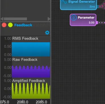
This Feedback window displays the raw input signal and the amplified signal together with the constant RMS value.

Basic EEG Classifier

Now that we know the basics of a classifier, we are ready to see an EEG classifier. This example runs a signal through two branches, with and without a low-pass filter. It shows the effect of the filter on the spectrum, then compares both branches with an amplitude threshold.

Test System (Pz)
├─> FFT ─> View
├─> IIR/FIR Filter
│   ├─> FFT ─> View
│   └─> Threshold
│       └─> Custom Feedback
│           (Activation With Filter)
└─> Threshold
    └─> Custom Feedback
        (Activation Without Filter)

Parameter (25)
└─> Thresh input of both
    Threshold nodes

Input

The input is the Test System node, in the Sensors category. It generates a simulated signal live from sine waves and random noise, at 128 Hz. It is not a recording and not EEG, but it has similar signal properties.

The Test System is only available while no other device is connected. It is removed as soon as a real device connects, so disconnect any real devices when you follow this example. The Test Devices entry in NMStudio > Settings > Devices > Drivers must also be on, which is the default, and your account must allow the device.

From this node we are interested in the Pz electrode (see 10-20 system). The Pz port connects directly to three other nodes: an FFT node, an IIR/FIR Filter node and a Threshold node.

Spectrum of the raw signal

The FFT node, in the DSP category, computes the fast Fourier transform of the signal, which maps the signal to the frequency domain.

Connect its Out (Spectrum) port to the In (Spectrum) port of a View node, in the Output category. Then open the window that shows the result, with Windows > Add > Spectrum View. None of the predefined layouts includes this window, so you see nothing until you add it. The window shows the magnitude of each frequency present in the signal.

With the defaults, FFT Order is 9, so each window has 512 samples. At 128 Hz this is 4 seconds of signal and a bin spacing of 0.25 Hz. Window Function is Hann. The node also subtracts the mean of each window before the transform, and there is no setting to turn this off.

In 1.7.3: The default FFT Order is 7, the Window Function setting is not applied, the mean is not subtracted and the magnitude scaling is different. Thresholds tuned on 1.7.3 spectra may behave differently in 1.8.2. See What changed since 1.7.3.

Low-pass filter

The second copy of the signal goes to an IIR/FIR Filter node, in the DSP category. Here it acts as a low-pass filter with a cut-off frequency of 5 Hz. Set these attributes:

• Filter Type: Lowpass, which is the default.
• Low Cut Frequency: 5 (the default is 7). Despite its name, this is the cut-off frequency of a low-pass filter. High Cut Frequency is hidden for this filter type.
• Filter Method: leave this on Butterworth. It is the only method implemented, and any other method gives no output.

Connect the filter to a second FFT and View pair. The Spectrum View window now shows both spectra. The filtered signal has much lower magnitudes for frequencies above 5 Hz.

Threshold

The Threshold node, in the Bio category, turns a signal into a decision. Its In port takes the signal to test. Its Thresh port takes the value to compare against. If Thresh is not connected, the node uses its Threshold attribute (default 0.5).

In 1.7.3: This attribute is labelled Low Threshold.

This example uses two Threshold nodes, one on the raw Pz signal and one on the filter output. A Parameter with Value 25 feeds the Thresh port of both, so you can move both thresholds together. Compare Function stays on its default, Greater than.

The node compares sample values, not the spectrum, so this is a threshold on signal amplitude. It has three outputs:

• % Passed: the fraction of samples in the last interval that passed, from 0 to 1. Interval Length sets the interval (default 1 second).
• Augment: 1 when the latest sample passes, otherwise 0.
• Inhibit: the opposite of Augment.

Connect each Augment output to a Custom Feedback node. Name them Activation Without Filter and Activation With Filter. These values fit the default range of 0 to 1, so no range change is needed. The Feedback window now shows when each branch is above the threshold.

To run a classifier in a session, see Running a session.